Particulate Nature of Matter

Understanding Matter and its Properties

Chemistry is fundamentally dedicated to comprehending matter and elucidating its diverse properties. This pursuit involves investigating the composition, structure, properties, and reactions of matter, ultimately aiming to explain the world around us at a fundamental level.

Evolution of Atomic Models: From Dalton to Thomson

Our understanding of the atom has evolved significantly over time, with various scientists proposing models to explain its structure. John Dalton, in 1808, proposed an atomic theory that laid the groundwork for modern chemistry, suggesting that matter is composed of indivisible atoms. Later, in 1904, J.J. Thomson introduced the "plum pudding" model, which depicted the atom as a sphere of uniformly distributed positive charge with negatively charged electrons embedded within it, much like plums in a pudding.

Rutherford's Nuclear Model of the Atom

Ernest Rutherford, through his groundbreaking gold foil experiment in 1911, revolutionized the atomic model. His observations led him to propose a nuclear model where the atom consists of a tiny, dense, positively charged nucleus at its center, with negatively charged electrons orbiting around it in a vast empty space. This model effectively disproved Thomson's "plum pudding" model.

Discovery of the Neutron and Subatomic Particles

The understanding of atomic structure was further refined with the discovery of the neutron. In 1932, James Chadwick identified the neutron, a neutral subatomic particle residing within the nucleus alongside protons. This discovery completed the picture of the three fundamental subatomic particles: protons (positively charged), electrons (negatively charged), and neutrons (no charge).

Representing Atoms with Nuclear Symbols

Protons and neutrons, collectively referred to as nucleons, are found within the atomic nucleus. The composition of an atom, specifically its number of protons and neutrons, is concisely represented by its nuclear symbol. This symbol provides crucial information about a specific isotope or nuclide.

Distinguishing Nuclear Symbols from Periodic Table Representations

It is crucial not to confuse the nuclear symbol with an element's representation on the periodic table. The nuclear symbol, also known as a nuclide symbol, specifically refers to a particular isotope and includes both the atomic number (Z), which represents the number of protons, and the mass number (A), which is the total number of protons and neutrons. In contrast, the periodic table typically displays the atomic number (Z) and the relative atomic mass (A_r). The relative atomic mass is a weighted average of the masses of all naturally occurring isotopes of an element, taking into account their relative abundances. It is defined as the ratio of the average mass of an atom of an element to one-twelfth of the mass of an atom of carbon-12, which is equivalent to the unified atomic mass unit.

Understanding Isotopes: Variations of an Element

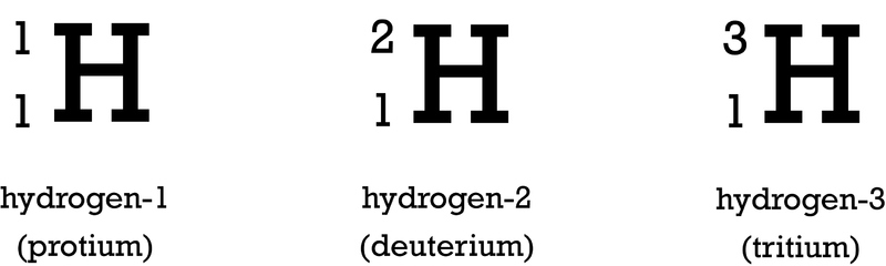
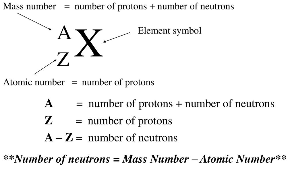
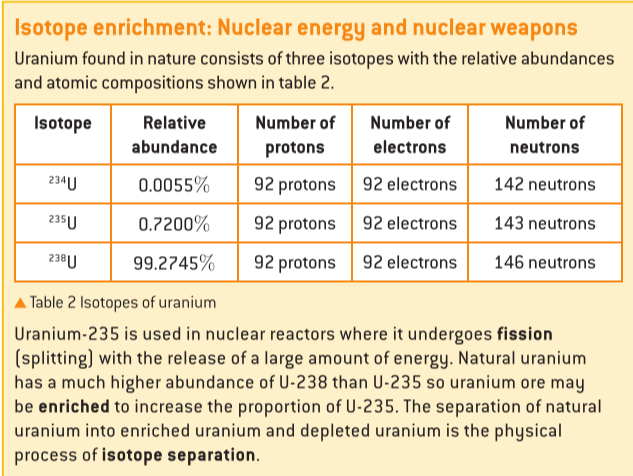
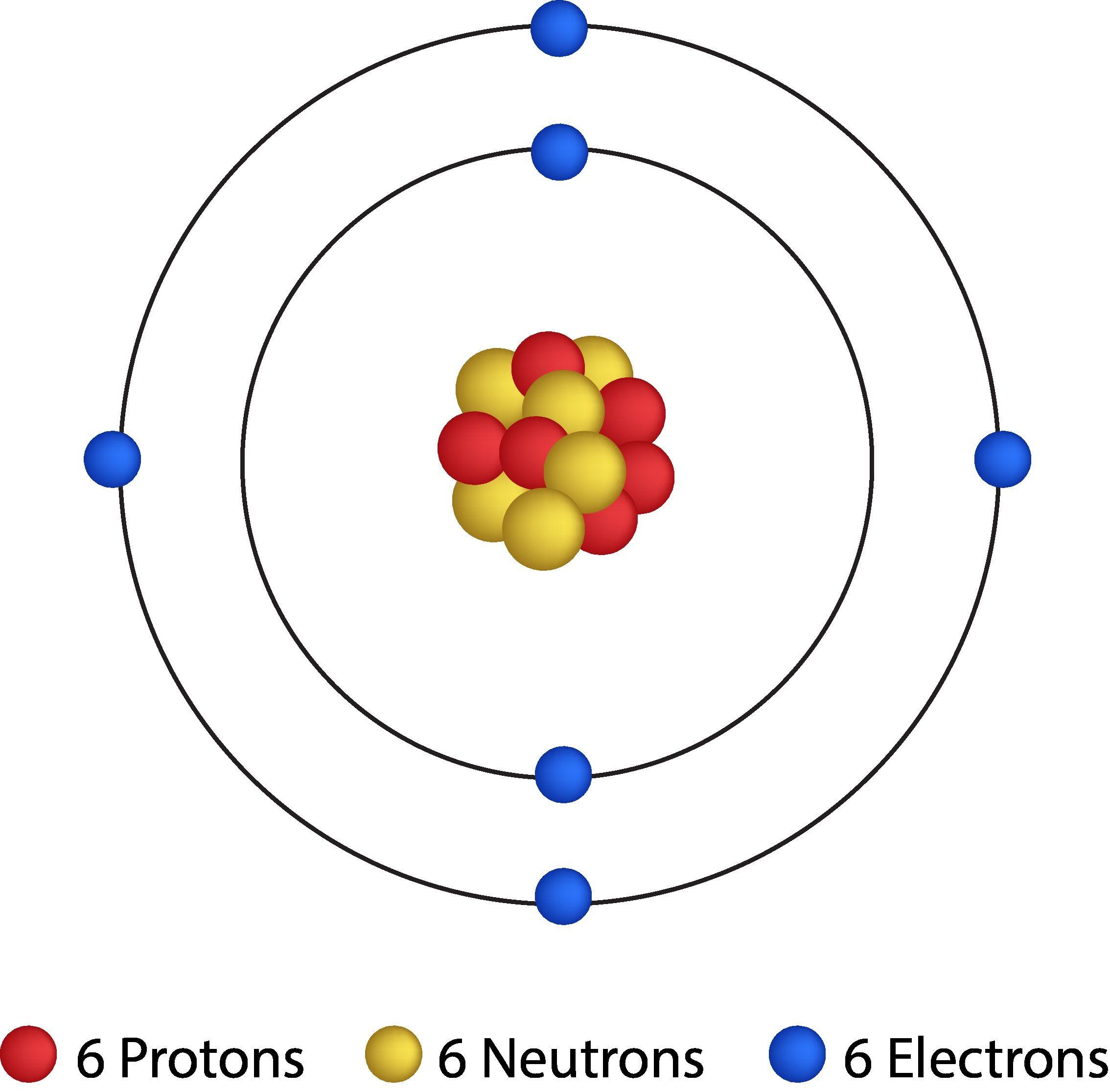
Isotopes are distinct forms of the same element, characterized by having an identical number of protons (atomic number, Z) but differing in their mass numbers (A) due to variations in their neutron count. Most elements naturally occur as a mixture of several isotopes. While isotopes of an element share identical chemical properties because their electron configurations (determined by the number of protons) are the same, they exhibit different physical properties, such as density and melting point, owing to their differing masses. For instance, uranium-235 (²³⁵U) is a crucial isotope used in nuclear reactors and weapons; however, natural uranium ore predominantly contains uranium-238 (²³⁸U), necessitating an enrichment process to increase the concentration of ²³⁵U through isotope separation techniques.

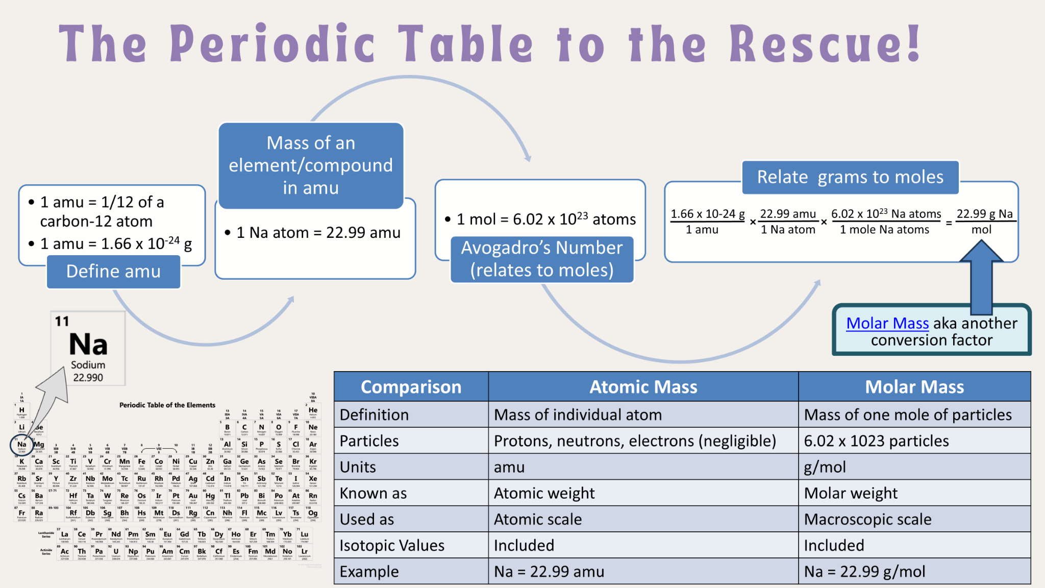
Defining Relative Atomic Mass

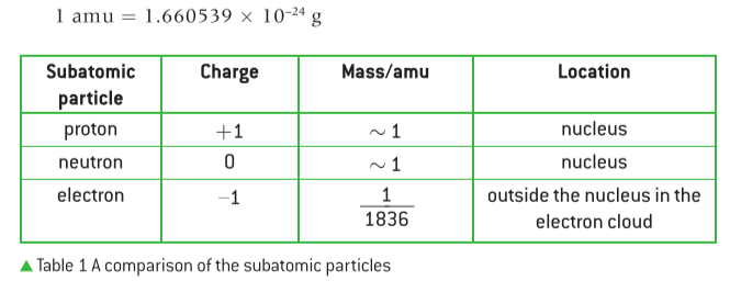
The relative atomic mass (A_r) of an element is a dimensionless quantity representing the ratio of the average mass of an atom of that element to the unified atomic mass unit. The mass of an atom is primarily determined by the combined mass of its protons and neutrons, as the mass of electrons is negligible in comparison. Given that the actual masses of individual atoms are exceedingly small, using relative atomic masses provides a more convenient and practical scale for chemical calculations. The unified atomic mass unit (amu or u) is defined as exactly 1/12th the mass of a single carbon-12 atom, with 1 amu being equivalent to 1.66005402 x 10^-27 kg. Since relative atomic masses are ratios, they are unitless. When referencing relative atomic masses from the IB Data Booklet, it is standard practice to express these values to two decimal places.

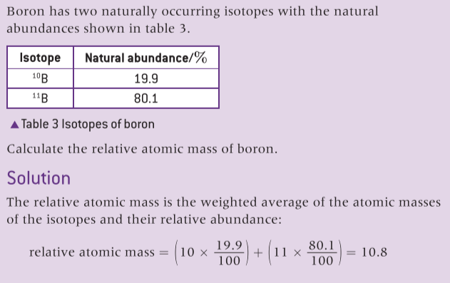
Calculating Relative Atomic Mass from Isotopic Abundance

The relative atomic mass of an element is a weighted average of the masses of its naturally occurring isotopes, taking into account their relative abundances.

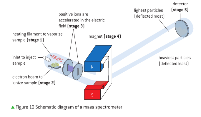
Measuring Atomic Mass and Isotopic Composition with Mass Spectrometry

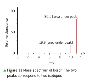
Mass spectrometry is a powerful analytical technique employed to measure the masses of atoms and molecules and determine the isotopic composition of elements. This method works by ionizing particles and then separating them based on their mass-to-charge ratio (m/z). The output of a mass spectrometer is a mass spectrum, where each peak corresponds to a specific isotope, and the height of each peak is directly proportional to the relative abundance of that isotope.

Determining Relative Atomic Mass from a Mass Spectrum

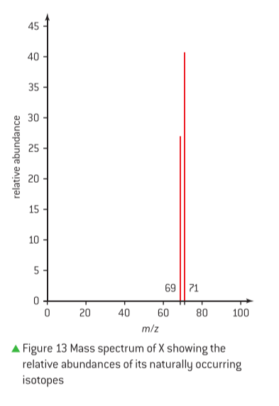
To deduce the relative atomic mass of an element from its mass spectrum, one must first determine the relative abundance of each isotope. For example, consider an element X with two isotopes, X-69 and X-71, as shown in a mass spectrum. If the peak height for X-69 is 27 and for X-71 is 41, the total area of the peak heights is 27 + 41 = 68. The relative abundance of each isotope can then be calculated:

• For X-69: (27 / 68) x 100 = 40%
• For X-71: (41 / 68) x 100 = 60%

The relative atomic mass is calculated by multiplying the mass of each isotope by its fractional abundance and summing these values: Relative atomic mass = (0.40 x 69) + (0.60 x 71) = 27.6 + 42.6 = 70.2. Rounding to an appropriate number of significant figures, typically determined by the precision of the given data, this value is approximately 70. By comparing this relative atomic mass to the periodic table, element X can be identified as Gallium (Ga). It is crucial to apply the correct number of significant figures when performing these mathematical calculations, as dictated by the problem's context.

The Nature of Electromagnetic Radiation

The electromagnetic spectrum, detailed in Section 3 of the data booklet, encompasses a wide range of radiation, each characterized by its energy, frequency, and wavelength. These properties are intrinsically linked: high-energy radiation corresponds to high frequency and short wavelength, while low-energy radiation is associated with low frequency and long wavelength. This inverse relationship between wavelength and frequency, and direct relationship between frequency and energy, is fundamental to understanding the behavior of light and other forms of electromagnetic radiation.

Understanding Atomic Emission Spectra

When atoms absorb energy, their electrons transition from their ground state to higher energy levels, becoming "excited." This excited state is unstable, and the electrons quickly return to lower energy levels, releasing the absorbed energy in the form of electromagnetic radiation. The specific wavelengths of light emitted by an element create a unique pattern known as its emission spectrum. Crucially, these spectra are not continuous; instead, they consist of discrete lines at particular wavelengths. Each line in an emission spectrum corresponds to the energy difference between two specific energy levels within the atom, providing a fingerprint for that element.

The Hydrogen Emission Spectrum and Quantized Energy Levels

The hydrogen atom, with its single electron, provides a clear illustration of quantized energy levels through its emission spectrum. While the visible portion of hydrogen's emission spectrum is well-known, it also produces lines in the ultraviolet (UV) and infrared regions, which are not visible to the naked eye. A key characteristic of all hydrogen emission spectra is that they consist of discrete lines that converge towards the high-energy (shorter wavelength) end of the spectrum. This convergence provides compelling evidence that the electron in a hydrogen atom can only occupy specific, fixed energy levels, rather than being able to exist at any arbitrary energy.

Principal Quantum Numbers and the Balmer Series

The energy levels within an atom are designated by the principal quantum number, *n*, which indicates both the energy level and the approximate size of the electron's orbital. For hydrogen, the visible emission spectrum, known as the Balmer series, arises specifically from electrons falling to the *n*=2 energy level from higher energy levels. As the value of *n* increases, the energy levels become progressively closer together. This phenomenon explains the observed convergence of lines in the emission spectrum at higher energies, as the energy differences between successive higher levels become smaller. For example, the following transitions result in visible light:

Transition	Wavelength (nm)
n=3 → n=2	656
n=4 → n=2	486
n=5 → n=2	434
n=6 → n=2	410

Visualizing the Balmer Series

The Balmer series is a prominent feature of the hydrogen emission spectrum, comprising the spectral lines that fall within the visible light range. These lines are a direct result of electron transitions from higher principal quantum numbers (*n* > 2) down to the *n*=2 energy level.

Bohr's Planetary Model of the Atom

Niels Bohr developed a mathematical model of the atom that successfully explained the discrete line spectra observed for various elements. A fundamental hypothesis of Bohr's model was that electrons occupy specific, quantized energy levels, often referred to as principal energy levels, around the atomic nucleus. Electrons situated further from the nucleus possess higher energy levels. According to Bohr's model, electrons typically reside in their lowest possible energy levels, known as the ground state. However, upon absorbing energy, these electrons can become "excited" and transition instantaneously to higher energy levels. A key aspect of this model is that electrons cannot exist in states between these defined energy levels; transitions are discrete jumps. This concept of quantized energy levels means that energy can only be absorbed or emitted in specific, fixed amounts or quantities.

The Quantum Model of the Atom

The quantum model represents the most current and accurate description of the atom. This model posits that electrons exist within a series of principal energy levels, typically seven, each of which is further subdivided into specific sublevels. Unlike Bohr's model, which described electrons orbiting in fixed paths, the quantum model describes the probability of finding an electron in a particular region around the nucleus.

Electron Orbitals

Within the quantum model, electron orbitals are defined as specific three-dimensional regions around the nucleus where there is a high probability of finding an electron. These orbitals have distinct shapes and energy levels, and they are fundamental to understanding chemical bonding and reactivity.

The Three States of Matter and Their Particulate Nature

Matter commonly exists in three primary states: solid, liquid, and gas. These states are distinguished by the arrangement and movement of their constituent particles. In a solid, particles are tightly packed in fixed positions, exhibiting only vibrational motion. Liquids have particles that are still close together but can move past one another, allowing them to flow and take the shape of their container. Gases, in contrast, have particles that are widely spaced and move randomly and rapidly, filling any available volume. The image below visually represents these distinct arrangements.

Temperature and Particle Kinetic Energy

Temperature is a fundamental macroscopic property that quantifies the average kinetic energy of the particles within a substance. A higher temperature indicates that the particles possess greater average kinetic energy, leading to more vigorous motion. The standard international (SI) unit for temperature is the Kelvin (K), which is directly related to the Celsius scale (°C) by the equation K = °C + 273.15. This relationship highlights that absolute zero (0 K) corresponds to -273.15 °C, the theoretical point at which all particle motion ceases. The images provided illustrate the concept of temperature and its measurement.

Energy Changes During Phase Transitions

When a substance undergoes a change of state, energy is either absorbed or released, but the temperature of the substance remains constant during the transition itself. Consider the heating of ice: as a sample of ice at -10 °C is heated, the water molecules absorb energy and vibrate more intensely. Upon reaching 0 °C, a solid-liquid equilibrium is established, and melting begins. During this phase, all the absorbed energy is utilized to overcome the attractive forces holding the water molecules in the crystal lattice, rather than increasing their kinetic energy, hence the temperature remains at 0 °C until all the ice has melted. Once all the ice has melted, the water molecules in the liquid state continue to absorb energy, causing them to vibrate faster and move with greater freedom, leading to an increase in temperature. This continues until 100 °C is reached, at which point a liquid-gas equilibrium is established, and boiling commences. Similar to melting, during boiling, the absorbed energy is used to overcome the intermolecular forces in the liquid state and convert it into a gas (steam), without a change in temperature. Only after all the liquid has been converted to steam can the temperature of the steam continue to rise. These phase changes are categorized by their energy exchange:

• Melting and boiling are endothermic processes, meaning they absorb energy from the surroundings.
• Conversely, freezing and condensation are exothermic processes, releasing energy to the surroundings.

Phase Change	Description	Energy Change
Melting	Solid to Liquid	Endothermic (absorbs energy)
Freezing	Liquid to Solid	Exothermic (releases energy)
Boiling/Vaporization	Liquid to Gas	Endothermic (absorbs energy)
Condensation	Gas to Liquid	Exothermic (releases energy)
Sublimation	Solid to Gas	Endothermic (absorbs energy)
Deposition	Gas to Solid	Exothermic (releases energy)

Understanding the Classification of Matter

Matter, the substance of which all physical objects are composed, can be broadly categorized based on its composition and properties. A fundamental distinction is made between pure substances and mixtures. Pure substances possess a uniform and definite composition, meaning their chemical makeup is consistent throughout and they have distinct properties. Mixtures, on the other hand, are combinations of two or more pure substances that are physically combined but not chemically bonded, and thus retain their individual properties. Pure substances are further divided into elements and compounds. Elements are the simplest forms of matter and cannot be broken down into simpler substances by chemical means. Each element is defined by the number of protons in its atoms. Compounds are pure substances formed when two or more different elements are chemically bonded together in fixed proportions. These chemical bonds result in a new substance with properties distinct from its constituent elements. Mixtures are classified as either homogeneous or heterogeneous. Homogeneous mixtures, also known as solutions, have a uniform composition and appearance throughout. The components are evenly distributed at a microscopic level, making it impossible to distinguish them visually. Examples include saltwater or air. Heterogeneous mixtures, conversely, have a non-uniform composition, and their components can be visually distinguished, often existing in separate phases. Examples include sand and water, or a salad.

Exploring Atomic Models with the PhET Simulator

The PhET simulator provides an interactive platform to visualize and understand fundamental concepts in chemistry, such as atomic structure and scattering experiments. Specifically, the Rutherford scattering simulation (available at http://phet.colorado.edu/sims/html/rutherford-scattering/latest/rutherford-scattering_en.html) allows for an exploration of the Rutherford model of the atom. The Rutherford model simulation demonstrates how alpha particles interact with a target atom. In this model, the atom is depicted as having a small, dense, positively charged nucleus at its center, surrounded by a cloud of negatively charged electrons. When alpha particles, which are positively charged, are fired at this atom, most pass straight through or are deflected only slightly, indicating that much of the atom is empty space. However, a small fraction of alpha particles are deflected at large angles, and some even bounce back, providing strong evidence for the existence of a concentrated positive charge within the atom – the nucleus. Changing the atom size in the simulation directly affects the scattering pattern of the alpha particles. A larger atom, while still mostly empty space, presents a larger target area for the alpha particles to interact with the electron cloud, potentially leading to more minor deflections. However, the core phenomenon of large-angle scattering due to the nucleus remains, as the size of the nucleus itself is not being altered in this specific parameter. The key takeaway is that the probability of a direct hit or close encounter with the nucleus, leading to significant deflection, is independent of the overall atomic radius, but rather dependent on the size and charge of the nucleus. Comparing the results of the Rutherford simulation to that of the Thomson's "plum pudding" model simulation reveals a stark contrast. In Thomson's model, the atom was envisioned as a sphere of uniformly distributed positive charge with electrons embedded within it, much like plums in a pudding. If this model were accurate, alpha particles would be expected to pass through with only minor deflections, as there would be no concentrated positive charge to cause large-angle scattering. The experimental observations, accurately represented by the Rutherford simulation, directly contradicted Thomson's model by showing significant deflections, thus leading to the development of the nuclear model of the atom.