Measurement & Uncertainties

The Inherently Probabilistic Nature of Chemistry

Chemistry offers profound insights into the material world, enabling us to comprehend its composition and interactions at a fundamental level. However, it is crucial to recognize that this understanding, while deep, does not equate to absolute certainty. As Brown and Ford eloquently state in their "Higher Level Chemistry" textbook, "Chemistry provides us with a deep understanding of the material world but it does not offer absolute certainty." This foundational principle underscores the importance of acknowledging the inherent limitations and probabilistic nature of scientific inquiry.

The Communal and Scrutinized Nature of Scientific Endeavor

The scientific enterprise is fundamentally communal, built upon the sharing of knowledge and the collective pursuit of understanding. This collaborative spirit necessitates that all scientific findings, including experimental data, are open to rigorous scrutiny through the process of peer review. This critical evaluation by other experts in the field ensures the validity, reliability, and reproducibility of research, fostering trust and progress within the scientific community.

The Inevitability of Measurement Uncertainties

A cornerstone of scientific measurement is the understanding that all measurements inherently possess uncertainties. These uncertainties arise from various factors, including limitations of instruments, experimental conditions, and human error. Consequently, these inherent uncertainties place legitimate limits on the conclusions that can be drawn from any given set of data. Recognizing and quantifying these uncertainties is not a weakness but rather a strength, as it allows for a more accurate and nuanced interpretation of results.

Uncertainty as a Catalyst for Scientific Progress

Far from being a hindrance, the recognition and careful consideration of uncertainties are vital for the advancement of science. By understanding the boundaries of our knowledge and the precision of our measurements, scientists can identify areas requiring further investigation, refine experimental techniques, and develop more sophisticated theories. This continuous cycle of measurement, uncertainty assessment, and refinement is what drives scientific progress forward.

Ethical Conduct in Scientific Research and Publication

Given the inherent uncertainties within the practice of science, it becomes paramount for scientists to exhibit specific behavioral characteristics when conducting and publishing their research. These include honesty, transparency, meticulousness in data collection and analysis, and a commitment to accurately reporting all findings, including their associated uncertainties. As J. Bronowski observed, "One aim of the physical sciences has been to give an exact picture of the material world. One achievement…has been to prove that this aim is unattainable." This profound statement implies that the aspiration of science should not be to achieve absolute certainty, but rather to continually refine our understanding, acknowledge limitations, and build a robust body of knowledge based on the most accurate and transparent data possible.

Quantifying Uncertainty in Laboratory Instruments

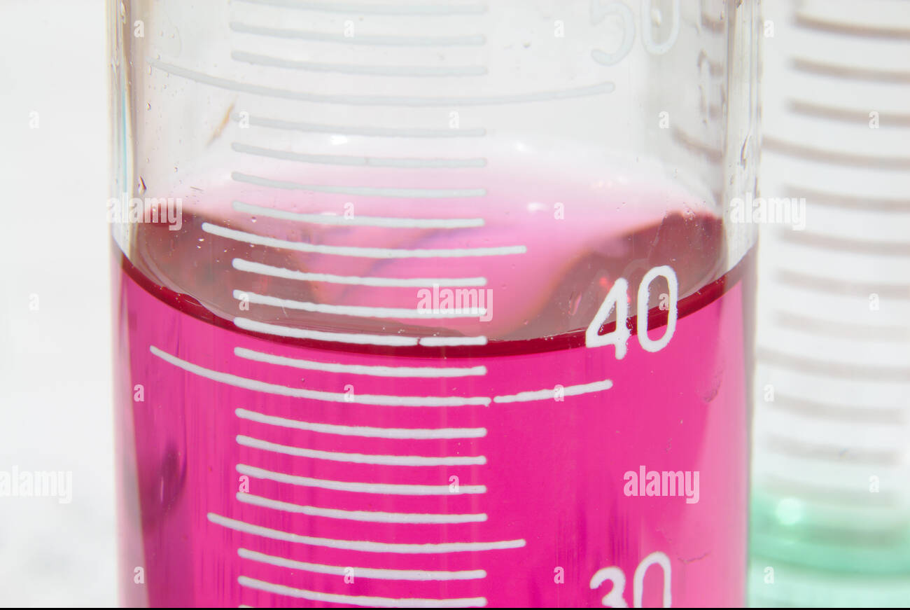
Different laboratory instruments inherently possess varying levels of uncertainty, which must be accounted for when reporting measurements. For instruments with an analogue scale, such as a graduated cylinder or a thermometer, the uncertainty is typically estimated as plus or minus (±) half of the smallest division marked on the scale. This acknowledges that a reading can reasonably fall anywhere within that half-division range.

In contrast, for digital scales, the last reported digit is considered uncertain. The uncertainty for a digital instrument is generally taken as plus or minus (±) the smallest scale division that the instrument can display. This means if a digital balance reads to two decimal places, its uncertainty would be ±0.01 units.

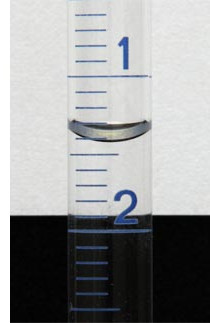
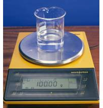
When reporting measurements, it is crucial to ensure that the precision of the reported value aligns with its associated uncertainty. For example, a measurement reported as 41.9 ± 0.5 mL indicates that the measurement is precise to the tenths place, consistent with the uncertainty. Similarly, 1.40 ± 0.05 mL is reported to the hundredths place, matching the uncertainty. A highly precise measurement like 100.00 ± 0.01 g is reported to the hundredths place, reflecting the very small uncertainty. It is also important to remember specific techniques for reading certain instruments, such as reading from the bottom of the meniscus for liquid volumes in glassware.

Acknowledging Non-Quantifiable Uncertainties

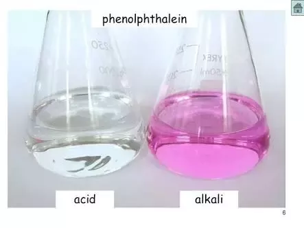
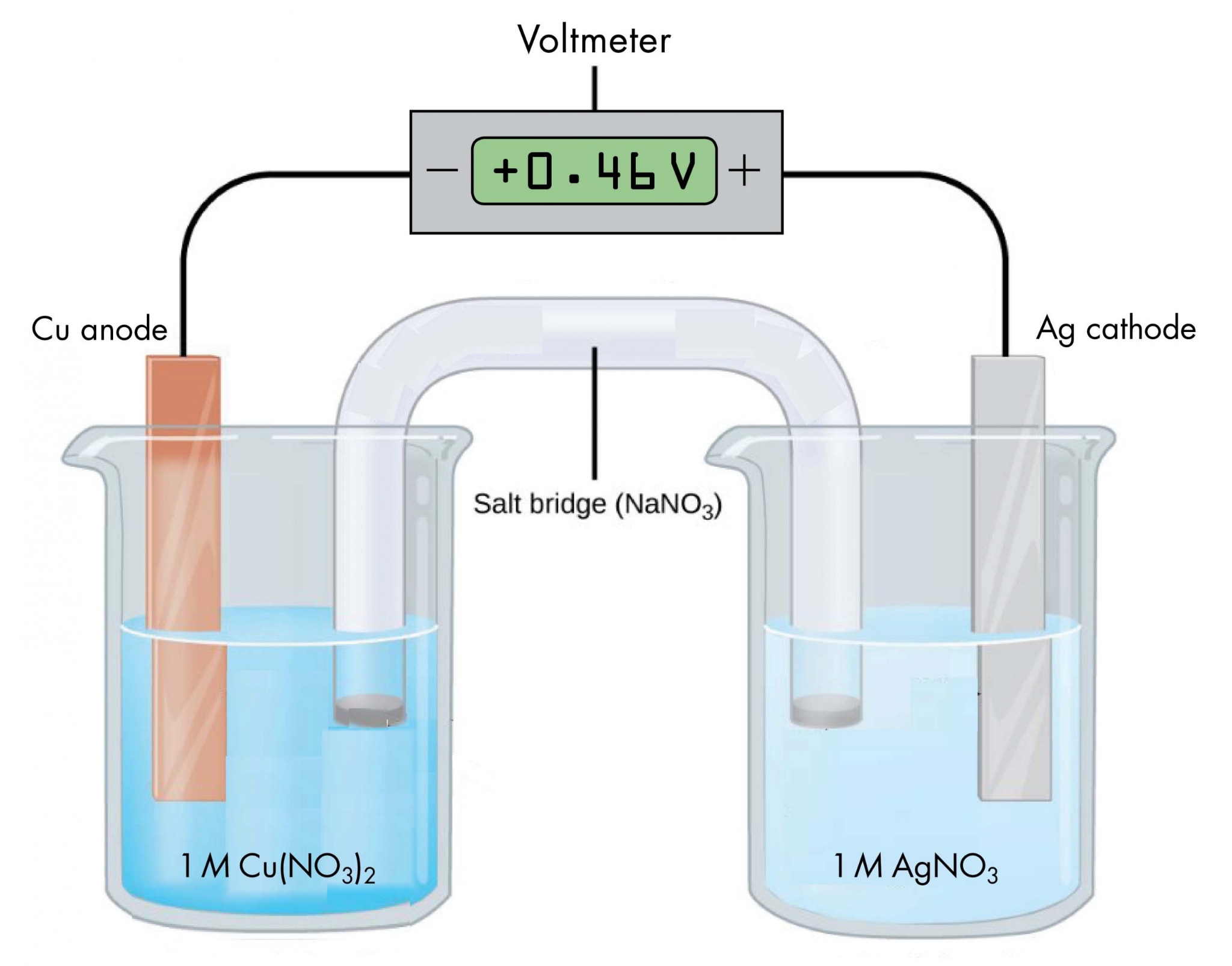
Beyond the inherent uncertainties of measuring instruments, other factors can introduce variability into experimental results. It is important to acknowledge all sources of uncertainty, even those that may not be easily quantifiable. These can include variations in time measurements, subjective interpretations such as changes in indicator colors during titrations, fluctuations in voltages of electrochemical cells, or temperature variations during thermodynamic reactions. While these may not always be expressed with a numerical ± value, their potential impact on the accuracy and precision of the experiment should be noted in any comprehensive analysis.

Understanding Uncertainty Through Significant Figures

Significant figures are crucial in scientific measurements as they convey the degree of uncertainty associated with a reported value. They represent all the digits in a measurement that are known with certainty, plus the first digit that is estimated or uncertain. It is essential to remember that all measurements must always be accompanied by appropriate units to provide context and meaning to the numerical value.

The Role of Scientific Notation in Reporting Significant Figures

When reporting measurements, especially those with many zeros, scientific notation becomes an invaluable tool for clearly indicating the correct number of significant figures. This method eliminates ambiguity regarding the significance of trailing zeros. For instance, a measurement of "1000 s" is ambiguous because the number of significant figures is unclear. However, expressing it in scientific notation, such as "1.000 × 10³ s", explicitly states that there are four significant figures, indicating a higher precision in the measurement. The following table illustrates how scientific notation clarifies the number of significant figures for a given measurement:

Measurement	Significant figures
1000 s	Unspecified
1 × 10³ s	1
1.0 × 10³ s	2
1.00 × 10³ s	3
1.000 × 10³ s	4

Similarly, for values less than one, scientific notation effectively communicates precision. Consider the concentration "0.45 mol dm⁻³". This value has two significant figures. When expressed in scientific notation as "4.5 × 10⁻¹ mol dm⁻³", the two significant figures are maintained. Adding trailing zeros after the decimal point in scientific notation, such as "4.500 × 10⁻¹ mol dm⁻³", explicitly increases the number of significant figures, thereby indicating greater precision in the measurement.

Measurement	Significant figures
0.45 mol dm⁻³	2
4.5 × 10⁻¹ mol dm⁻³	2
4.50 × 10⁻¹ mol dm⁻³	3
4.500 × 10⁻¹ mol dm⁻³	4
4.5000 × 10⁻¹ mol dm⁻³	5

Categorization of Experimental Errors

Experimental errors, which are inevitable in any scientific measurement, can be broadly classified into two main categories: random errors and systematic errors. Understanding the distinction between these types of errors is crucial for evaluating the reliability of experimental results and for designing effective strategies to minimize their impact.

Understanding Random Errors

Random errors arise from unpredictable fluctuations in experimental conditions or from the inherent limitations of measurement. These errors have multiple potential causes, including subtle changes in the surrounding environment such as temperature variations or air currents, slight misinterpretations of measurement readings by the experimenter, or simply an insufficient amount of collected data. A defining characteristic of random errors is that they have an equal probability of causing a measurement to be either too high or too low relative to the true value. While individual random errors cannot be eliminated, their overall impact on the experimental outcome can be significantly reduced by repeating the experiment multiple times and averaging the results. This practice helps to cancel out the random fluctuations, leading to a more precise measurement.

The Nature of Systematic Errors

In contrast to random errors, systematic errors consistently bias measurements in one direction, meaning they will always make the result either too high or too low. These errors typically stem from flaws in the experimental design, the procedure followed, or the calibration of the instruments used. Because systematic errors are inherent to the experimental setup, simply repeating the experiment multiple times will not reduce them; the same error will be consistently reproduced. To mitigate systematic errors, the experimental design or procedure itself must be modified. A key indicator of a systematic error is a consistent difference between the recorded experimental value and the accepted literature value for a given quantity.

Ensuring Repeatability and Reproducibility

To assess the reliability of experimental data, it is considered good scientific practice to ensure both repeatability and reproducibility. Repeatability refers to the ability of the same experimenter, using the same equipment and conditions, to obtain consistent results when duplicating an experiment. Reproducibility, on the other hand, refers to the ability of different experimenters, using different equipment or in different laboratories, to obtain similar results when performing the same experiment. These practices help to identify and quantify the extent of random errors.

Consider an example where the mass of a piece of magnesium ribbon is measured multiple times, yielding the following results: 0.1234 g, 0.1232 g, 0.1233 g, 0.1234 g, 0.1235 g, and 0.1236 g. The average mass is calculated as (0.1234 + 0.1232 + 0.1233 + 0.1235 + 0.1236) / 5 = 0.1234 g. To express the uncertainty associated with these measurements, we can calculate the range of the data, which is the difference between the highest and lowest values (0.1236 g - 0.1232 g = 0.0004 g). The uncertainty is then half of this range, so 0.0004 g / 2 = 0.0002 g. Therefore, the average mass can be reported as 0.1234 ± 0.0002 g, indicating that the data spans a range of ±0.0002 g from the average. This uncertainty primarily reflects the impact of random errors on the precision of the measurement.

Identifying and Correcting Systematic Errors

Systematic errors, unlike random errors, consistently skew results in a particular direction. For instance, if the mass of a magnesium ribbon is measured several times, but the balance was not correctly zeroed, all readings would be consistently higher or lower than the true value. If the readings obtained were 0.1236 g, 0.1234 g, 0.1235 g, 0.1236 g, 0.1237 g, and 0.1238 g, and it was later discovered that the balance was consistently reading 0.0002 g too high, then all recorded values would be systematically inflated by that amount. The average mass would be (0.1236 + 0.1234 + 0.1235 + 0.1237 + 0.1238) / 5 = 0.1236 g, with an uncertainty of ± 0.0002 g. However, even with this precision, the result is inaccurate due to the systematic offset.

Common examples of systematic errors include:
    • Incorrectly reading the volume of a liquid from the top of the meniscus instead of the bottom, leading         to consistently higher volume readings.
    • Consistently overshooting the endpoint in a titration, resulting in an overestimation of the volume of           titrant delivered.
• Using instruments that have not been properly calibrated, causing all measurements to be consistently off by a certain amount.

The presence of a systematic error is primarily detected by its effect on the accuracy of an experiment, meaning how close the measured value is to the true or accepted value.

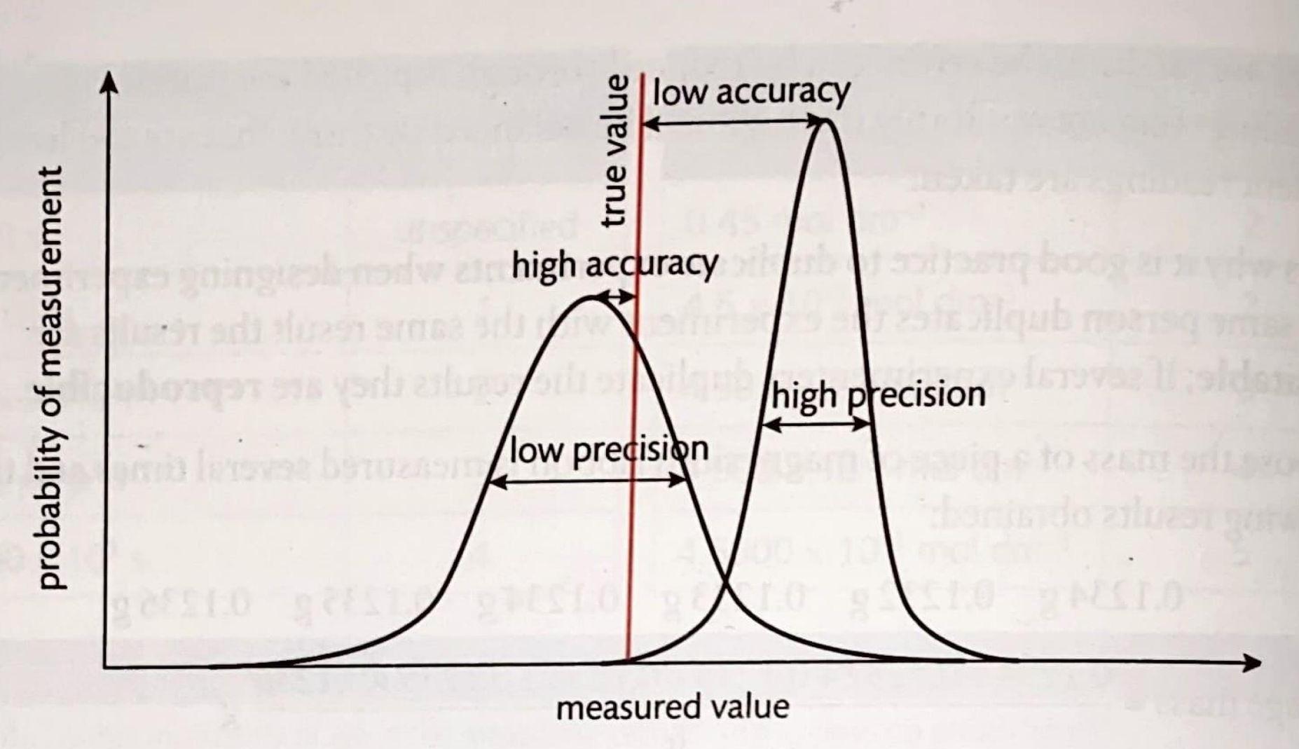
Distinguishing Accuracy from Precision

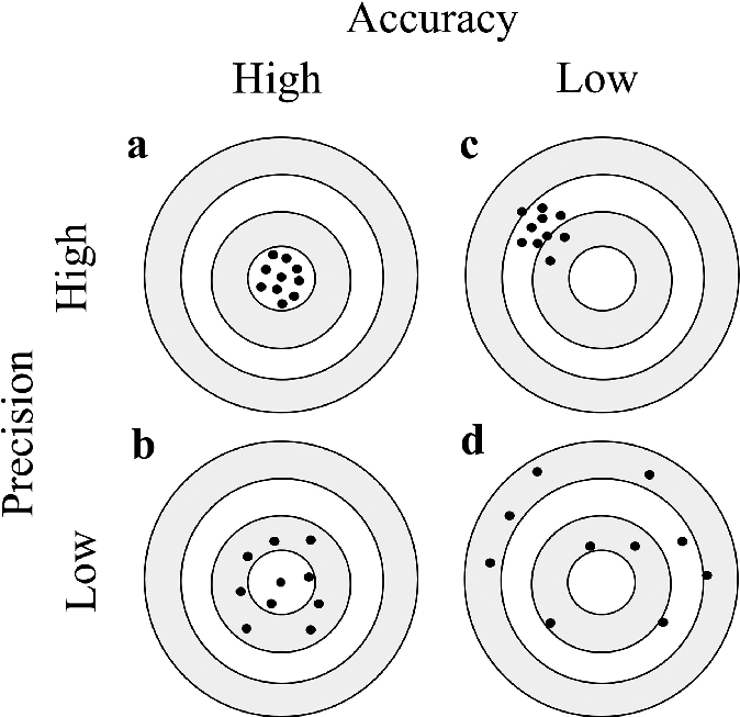
Accuracy and precision are two fundamental concepts in experimental measurements that are often confused but refer to distinct aspects of data quality. Accuracy describes how close a measured value is to the true or accepted value. A smaller systematic error directly leads to greater accuracy. Precision, on the other hand, refers to how close repeated measurements are to each other, regardless of their proximity to the true value. A smaller random error contributes to greater precision, indicating that the results are highly reproducible.

The relationship between accuracy and precision can be visualized as follows:

Characteristic	Accuracy	Precision
Affected by	Systematic errors	Random errors
Definition	Closeness of a measurement to the accepted value	Closeness of repeated measurements to each other
Improvement method	Changing experimental design/procedure	Repeating experiments and averaging results

Expressing Measurement Uncertainty

When reporting experimental data, it is crucial to quantify the associated uncertainty. This uncertainty can be expressed in several ways: as an absolute uncertainty, a fractional uncertainty (also known as relative uncertainty), or a percentage uncertainty. Absolute uncertainty represents the actual range of possible values for a raw measurement, typically expressed in the same units as the measurement itself. Fractional uncertainty is calculated by dividing the absolute uncertainty by the measured value, providing a unitless ratio that indicates the uncertainty relative to the magnitude of the measurement. Percentage uncertainty takes this a step further by multiplying the fractional uncertainty by 100%, expressing the uncertainty as a percentage of the measured value.

Distinguishing Percentage Uncertainty from Percentage Error

It is important to differentiate between percentage uncertainty and percentage error, as they represent distinct concepts in experimental analysis. Percentage uncertainty quantifies the precision of a measurement, reflecting the inherent limitations of the measuring instrument and the experimental technique. In contrast, percentage error assesses the accuracy of an experimental result by comparing it to a known or accepted value. The formula for percentage error is given by the absolute difference between the accepted value and the experimental value, divided by the accepted value, and then multiplied by 100%. This calculation provides an indication of how close the experimental result is to the true value.

Calculating Percentage Uncertainty: An Example

Consider a raw data measurement reported as 23.4 mol dm⁻³ ± 0.2 mol dm⁻³. Here, 0.2 mol dm⁻³ represents the absolute uncertainty. To calculate the fractional uncertainty, we divide the absolute uncertainty by the measured value: 0.2 mol dm⁻³ / 23.4 mol dm⁻³. This yields approximately 0.0085. To convert this to a percentage uncertainty, we multiply by 100%, resulting in an uncertainty of 0.85%.

Significant Figures in Uncertainty Reporting

When performing calculations involving uncertainties, it is a critical practice to avoid rounding intermediate values. Rounding too early can introduce imprecision into the final result. Once the final uncertainty is calculated, specific rules apply to the number of significant figures used for reporting. If the calculated percentage uncertainty is 2% or greater, it should be reported to one significant figure. However, if the calculated percentage uncertainty is less than 2%, it should be reported to two significant figures. This convention ensures that the reported uncertainty appropriately reflects the precision of the measurement.

Propagating Uncertainties in Experimental Data

When processing experimental data, it is crucial to account for the uncertainties present in the raw measurements. These uncertainties must be propagated consistently through any calculations to ensure that the final calculated result accurately reflects the precision of the original measurements.

Uncertainty Propagation in Addition and Subtraction

For operations involving addition or subtraction, the absolute uncertainty of the final result is determined by summing the absolute uncertainties of the individual measurements. For example, consider two burette readings: an initial reading of 15.05 ± 0.05 cm³ and a final reading of 37.20 ± 0.05 cm³. To find the volume delivered, we subtract the initial reading from the final reading: 37.20 cm³ - 15.05 cm³ = 22.15 cm³. The absolute uncertainty of the delivered volume is the sum of the individual absolute uncertainties: 0.05 cm³ + 0.05 cm³ = 0.10 cm³. Therefore, the reported value for the volume delivered would be 22.15 ± 0.10 cm³.

Uncertainty Propagation in Multiplication and Division

When performing multiplication or division, the percentage uncertainties of the individual measurements are added to determine the total percentage uncertainty of the final result. This total percentage uncertainty can then be used to calculate the absolute uncertainty of the final value. For instance, when calculating density, if the mass is 24.0 g ± 0.5 g and the volume is 2.0 cm³ ± 0.1 cm³, we first determine the percentage uncertainty for each measurement.

Value	Absolute uncertainty
Mass (g)	24.0
Volume (cm³)	2.0

The density is calculated as mass divided by volume: 24.0 g / 2.0 cm³ = 12 g cm⁻³. To find the total percentage uncertainty, we add the individual percentage uncertainties: 2% + 5% = 7%. Finally, we calculate the absolute uncertainty of the density by taking 7% of the calculated density: 0.07 × 12 g cm⁻³ = 0.84 g cm⁻³. Rounding to one significant figure, the absolute uncertainty is 0.8 g cm⁻³. Therefore, the density would be reported as 12 ± 0.8 g cm⁻³.

Value	Absolute uncertainty
Density (g cm⁻³)	12 (2 sig figs)

Summary of Uncertainty Propagation Rules

In summary, the method for propagating uncertainties depends on the mathematical operation performed:

• For measurements that are added or subtracted, the total absolute uncertainty is found by summing the individual absolute uncertainties.
• For measurements that are multiplied or divided, the total percentage uncertainty is found by summing the individual percentage uncertainties. This total percentage uncertainty is then used to calculate the total absolute uncertainty of the final result.

Precision in Addition and Subtraction

When performing addition or subtraction with measured values, the precision of the result is determined by the measurement with the fewest decimal places. This means that the final answer cannot be more precise than the least precise measurement used in the calculation. For instance, if we add two masses, 1.21 g (with two decimal places) and 0.56 g (also with two decimal places), the total mass of 1.77 g will also be reported to two decimal places. Similarly, when calculating a temperature change from 25.2 °C to 34.2 °C, both measurements have one decimal place, so the difference, 9.0 °C, is also reported to one decimal place. A common mistake is to report more decimal places than the least precise measurement allows. For example, if 50 g of water (no decimal places specified, implying precision to the nearest gram) is added to 1.00 g of sugar (two decimal places), the total mass is 51 g, not 51.00 g, because the precision is limited by the 50 g measurement.

Precision in Multiplication and Division

For calculations involving multiplication or division, the number of significant figures dictates the precision of the final answer. The result should be rounded to have the same number of significant figures as the measurement with the fewest significant figures. Consider the example of determining the density of sodium chloride. If the mass is 5.00 g (three significant figures) and the volume is 2.3 cm³ (two significant figures), the calculated density will be 2.173913043 g cm⁻³. However, since the volume measurement has only two significant figures, the density must be rounded to two significant figures, resulting in 2.2 g cm⁻³. When dealing with uncertainties in multiplication and division, it is often useful to consider percentage uncertainties. The percentage uncertainty for mass (0.01/5.00) is 0.2%, and for volume (0.1/2.3) is approximately 4%. These percentage uncertainties are then added to find the total percentage uncertainty, which in this case is 4.2%. This combined percentage uncertainty can then be used to determine the absolute uncertainty of the final calculated value. For the density example, the absolute uncertainty would be approximately 0.1 g cm⁻³.

Operation	Rule for Significant Figures
Addition/Subtraction	The result should have the same number of decimal places as the measurement with the fewest decimal places.
Multiplication/Division	The result should have the same number of significant figures as the measurement with the fewest significant figures.

Impact of Individual Uncertainties on Overall Results

When conducting experiments, it is crucial to understand how individual measurements contribute to the overall uncertainty of the final result. If one particular measurement possesses a significantly higher uncertainty compared to others, it will disproportionately influence the total uncertainty of the calculated outcome. For instance, in many calorimetric experiments, the temperature measurement obtained from thermometers often introduces the largest uncertainty. Recognizing this can guide experimental design, suggesting that more repetitions of the experiment, or the use of more precise temperature-measuring devices, might be necessary to improve the reliability of the results.

Identifying and Addressing Systematic Errors

Discrepancies between experimental results and accepted literature values can often point towards systematic errors in the experimental design. For example, if the enthalpy change (ΔH) measured for an exothermic reaction is consistently lower than the established literature value, it strongly suggests that heat is being lost to the surroundings. This heat loss represents a systematic error, as it consistently biases the results in one direction. Identifying such systematic errors is a critical step in refining experimental procedures. It necessitates an alteration in the experimental design, perhaps by improving insulation, using a more accurate calorimeter, or accounting for heat capacity of the apparatus, to minimize heat exchange with the environment and obtain more accurate data.

Fundamentals of Data Visualization in Chemistry

In chemistry, graphs are indispensable tools for visually representing and understanding the relationships between different variables. When constructing a graph, it is crucial to correctly identify and place the independent and dependent variables. The independent variable, which is the factor that is intentionally changed or controlled in an experiment, is always plotted on the x-axis. Conversely, the dependent variable, which is the factor that is measured or observed in response to changes in the independent variable, is always plotted on the y-axis.

For most chemical data, a scatter plot is the most appropriate type of graph, accounting for approximately 99% of graphical representations in the field. When setting up the axes, it is important to use even intervals, though different scales can be applied to the x and y axes to best represent the data. The goal is to ensure that the data points occupy the majority of the graph's space, maximizing clarity and readability.

To quantify the strength and direction of the relationship between variables, two key statistical measures are employed: the correlation coefficient (r) and the coefficient of determination (R²). The correlation coefficient (r) provides a numerical value that indicates both the magnitude and direction of the linear relationship between two variables. A value of r close to +1 or -1 signifies a strong linear relationship, while a value close to 0 indicates a weak or no linear relationship. For instance, an r value of 0.99 suggests a very strong positive linear correlation.

A trendline, also known as a line of best fit, is a visual representation of the general pattern and direction of the data points on a scatter plot. The equation of this trendline is particularly useful as it allows for both interpolation (estimating values within the range of the observed data) and extrapolation (predicting values outside the range of the observed data). The coefficient of determination (R²) further elaborates on the relationship by indicating the proportion of the variance in the dependent variable that can be explained by the independent variable. R² values range from 0 to 1, with values closer to 1 suggesting that the independent variable accounts for a large portion of the variation in the dependent variable. Conversely, R² values closer to zero imply that other uncontrolled variables or experimental error might be significantly contributing to the observed changes in the dependent variable.

Interactive Data Analysis

For a more dynamic exploration of data plotting and analysis, an interactive whiteboard is available. This tool facilitates group discussions and allows for real-time manipulation and visualization of data sets.

Click the picture to go to the interactive whiteboard

Illustrative Examples of Correlation Types

Graphs can exhibit various types of correlations, each providing unique insights into the relationship between variables. A positive correlation indicates that as the independent variable increases, the dependent variable also tends to increase. Conversely, a negative correlation means that as the independent variable increases, the dependent variable tends to decrease. The strength of these correlations can be categorized as strong, moderate, or weak, depending on how closely the data points cluster around the trendline.

A strong correlation is characterized by very little variance in the dependent variable with respect to the independent variable, suggesting a robust relationship. A moderate correlation shows a noticeable but not extreme amount of variance, indicating a relationship that is present but less precise. Finally, a weak correlation implies a large amount of variance, suggesting a tenuous or inconsistent relationship between the variables.

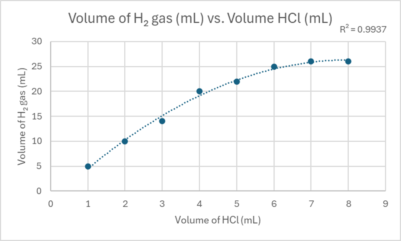
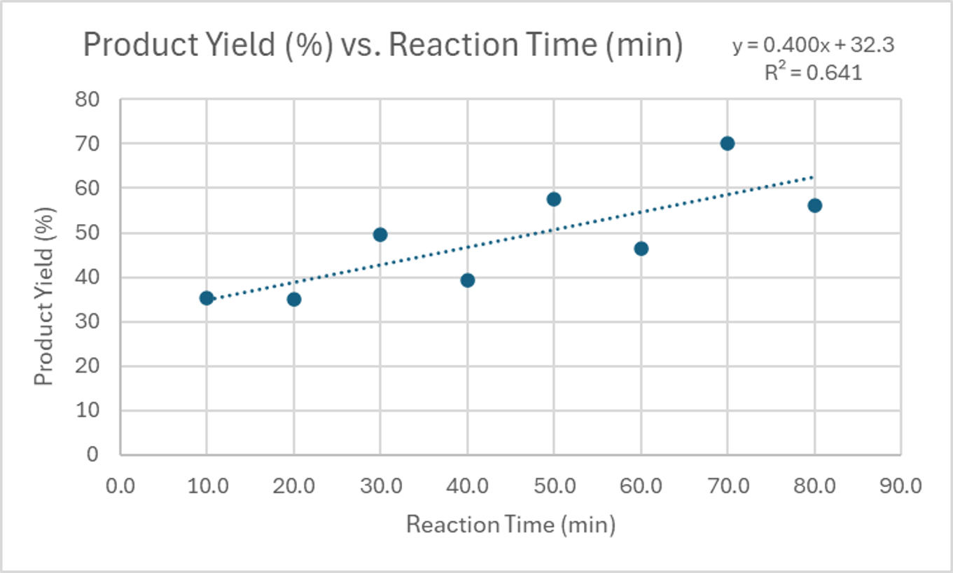
For instance, a strong, non-linear, positive correlation might be observed in a reaction where the product yield initially increases rapidly with temperature but then plateaus. A moderate, linear, positive correlation could be seen in a titration where the volume of reactant added directly corresponds to a steady increase in a measured property. The following tables provide data that can be used to visualize these different types of correlations.

Further Examples of Correlation Patterns

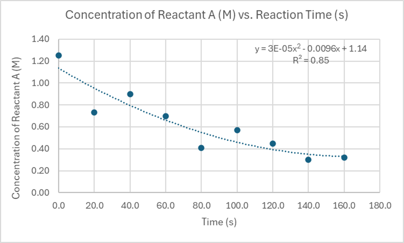
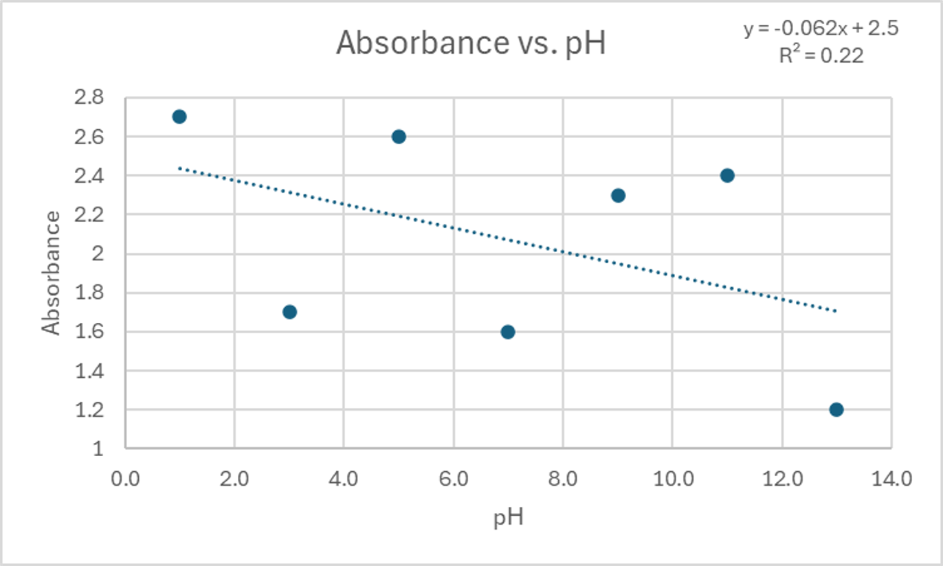
Continuing our exploration of correlation types, a strong, non-linear, negative correlation might be observed in a decay process where the concentration of a reactant decreases rapidly at first and then more slowly over time. A weak, negative correlation could be present in a scenario where an increase in one variable generally leads to a decrease in another, but with considerable scatter in the data points.

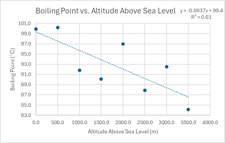
Distinguishing Between Moderate and No Correlation

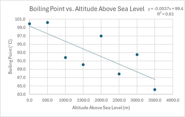
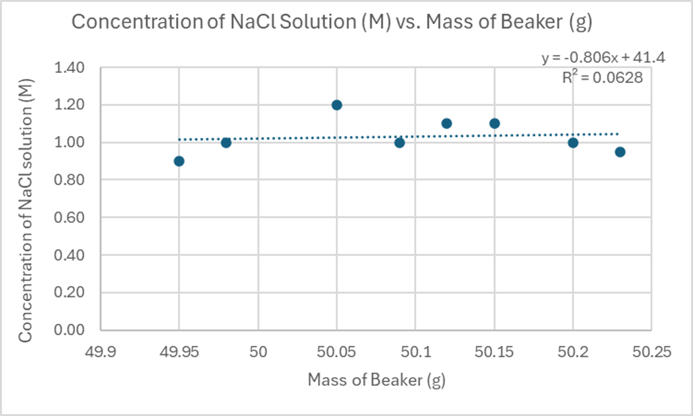
A moderate, linear, negative correlation would show a general downward trend as the independent variable increases, but with the data points not perfectly aligned along a straight line. In contrast, a scenario with no significant correlation implies that there is such a large amount of variance in the dependent variable that no discernible relationship with the independent variable can be established. In such cases, the data points appear randomly scattered, and a trendline would not accurately represent any underlying pattern.

Interpreting Correlation Coefficients

The correlation coefficient (r) is a quantitative measure that describes how strongly two variables are related to each other. Its value ranges from -1 to +1. A perfect correlation, either positive (+1) or negative (-1), indicates that all data points lie perfectly on a straight line. As the absolute value of r decreases towards 0, the strength of the correlation weakens.

While the boundaries between different correlation strengths can be subjective, a general rule of thumb for interpreting r values is as follows:• • • • •

• Perfect Correlation: r = +1 or r = -1
• Strong Correlation: r values typically between +0.8 and +1.0, or -0.8 and -1.0
• Moderate Correlation: r values typically between +0.4 and +0.8, or -0.4 and -0.8
• Weak Correlation: r values typically between +0.2 and +0.4, or -0.2 and -0.4
• No Correlation: r values close to 0 (e.g., between -0.2 and +0.2)

It is important to remember that a positive correlation means both variables increase or decrease together, while a negative correlation means one variable increases as the other decreases. The coefficient of determination (R²), which is the square of the correlation coefficient, provides further insight. R² values closer to zero suggest that a significant portion of the variance in the dependent variable is not explained by the independent variable, implying that other uncontrolled variables or experimental error may be contributing factors. R² values always range from 0 to 1.

Distinguishing Between Correlation Coefficient and Coefficient of Determination

The correlation coefficient (r) and the coefficient of determination (R²) are both statistical measures used to assess the relationship between two variables, typically within the context of linear models. The correlation coefficient quantifies both the strength and the direction of a linear relationship, ranging from -1 to +1. A value of +1 indicates a perfect positive linear correlation, -1 indicates a perfect negative linear correlation, and 0 indicates no linear correlation. Conversely, the coefficient of determination (R²) indicates the proportion of the variance in the dependent variable that can be predicted from the independent variable. Its range is from 0 to 1, where 1 signifies that the model perfectly predicts the observed data, and 0 means the model explains none of the variability. It is important to note that R² is the square of r, but if r is negative or less than 1, R² may be smaller than r. Therefore, the statement that the coefficient of determination is always greater than the correlation coefficient, regardless of the data, is incorrect. Furthermore, both coefficients are primarily applied to linear models, making the assertion that the correlation  coefficient is used in nonlinear modeling while the coefficient of determination is exclusive to linear regression also inaccurate. 

Interpreting Scientific Data: Correlation Versus Causation

When analyzing scientific data, it is crucial to understand that data does not definitively "prove" anything in an absolute sense. Instead, scientific data serves to either support or refute a given hypothesis. There is no absolute "truth" in science; rather, our understanding evolves as more evidence is gathered. A fundamental principle in data interpretation is that correlation does not imply causation. While two variables may exhibit a strong statistical correlation, this relationship does not automatically mean that one variable directly causes a change in the other. There could be confounding variables, coincidental relationships, or an entirely different underlying cause influencing both variables.