Electronic Configuration

Introduction to the Electromagnetic Spectrum

The electromagnetic spectrum encompasses the entire range of electromagnetic radiation, which is a form of energy that propagates through space as waves. This fundamental concept is detailed in Section 5 of the IB Chemistry data booklet. Understanding the electromagnetic spectrum is crucial for comprehending various chemical phenomena, including spectroscopy and the interaction of light with matter.

Relationship Between Energy, Frequency, and Wavelength

A key characteristic of electromagnetic radiation is the inverse relationship between its energy and wavelength, and a direct relationship between its energy and frequency. High-energy electromagnetic radiation is characterized by high frequency and short wavelengths. Conversely, low-energy radiation exhibits low frequency and long wavelengths. This relationship is mathematically described by the Planck-Einstein relation (E = hf) and the wave equation (c = λf), where E is energy, h is Planck's constant, f is frequency, c is the speed of light, and λ is wavelength.

The Origin of Emission Spectra

When atoms absorb energy, their electrons can transition from their ground state to higher energy levels, becoming "excited." However, this excited state is unstable. To return to a more stable configuration, these excited electrons release the absorbed energy by falling back to lower energy levels. This emitted energy is in the form of electromagnetic radiation. Crucially, each element possesses a unique electron configuration and thus a distinct set of energy levels. Consequently, when electrons in a particular element de-excite, they produce a characteristic emission spectrum, which acts like a fingerprint for that element. These emission spectra are not continuous; instead, they consist of discrete lines at specific wavelengths, indicating that electrons can only occupy certain quantized energy levels within an atom. Each line in the spectrum corresponds to the energy difference between two specific energy levels.

The Quantized Nature of the Hydrogen Emission Spectrum

While the visible emission spectrum of hydrogen is well-known, hydrogen also produces emission spectra in other regions of the electromagnetic spectrum, such as the ultraviolet (UV) and infrared (IR) regions, which are not perceptible to the naked eye. A fundamental characteristic of all these spectra is the presence of discrete lines that exhibit a phenomenon called convergence: the lines get progressively closer together towards the higher energy (shorter wavelength) end of the spectrum. This observation provides compelling evidence that the electron in a hydrogen atom can only exist in specific, fixed energy levels, rather than being able to occupy any arbitrary energy.

Principal Quantum Number and the Balmer Series

The energy levels within an atom are designated by the principal quantum number, *n*, which also indicates the approximate size of the electron's orbital. For hydrogen, the visible emission spectrum, known as the Balmer series, arises specifically when electrons transition from higher energy levels down to the *n*=2 energy level. As the value of *n* increases, meaning the electron is in a higher energy level, the energy levels themselves become progressively closer together. This decreasing energy difference between successive higher energy levels is directly responsible for the convergence of the spectral lines observed in the emission spectrum. For example, the following transitions contribute to the visible Balmer series:

Transition	Wavelength
n=3 → n=2	656 nm
n=4 → n=2	486 nm
n=5 → n=2	434 nm
n=6 → n=2	410 nm

Visualizing the Balmer Series

The Balmer series, as discussed, represents the set of spectral lines in the visible region of the electromagnetic spectrum that result from electron transitions to the *n*=2 energy level in a hydrogen atom.

Principal Energy Levels and Electron Capacity

Electrons within an atom are organized into distinct main energy levels, often referred to as shells. These shells are designated by the principal quantum number, 'n', which can take on integer values (n = 1, 2, 3, and so on). Each main energy level has a fixed maximum capacity for electrons, determined by the formula 2n². For instance, the first energy level (n=1) can hold a maximum of 2(1)² = 2 electrons, while the second energy level (n=2) can accommodate 2(2)² = 8 electrons.

Sub-levels and Electron Distribution

Within each main energy level, electrons are further distributed among sub-levels, also known as subshells. Each sub-level has a specific shape and can hold a fixed number of electrons, which is dependent on the number of orbitals it contains. The types of sub-levels present increase with the principal quantum number. The following table illustrates the sub-levels found within the first four main energy levels and their respective maximum electron capacities:

Level	Sub-levels (with max. number of electrons in each)
n = 1	s (2)
n = 2	s (2) and p (6)
n = 3	s (2), p (6), and d (10)
n = 4	s (2), p (6), d (10), and f (14)

Electron Occupancy in Orbitals

Electrons reside in specific regions of space called orbitals, which are located within these discrete energy levels. Each individual orbital has a limited capacity, capable of holding a maximum of two electrons. A crucial aspect of electron behavior within an orbital is that these two electrons must possess opposite spins, a principle known as the Pauli Exclusion Principle. This opposite spin creates a magnetic moment that allows them to coexist within the same orbital without violating quantum mechanical rules.
 

Defining Atomic Orbitals and the Uncertainty Principle

The concept of an atomic orbital is fundamentally linked to Heisenberg's Uncertainty Principle, which states that it is impossible to simultaneously know both the exact position and the exact momentum (and thus velocity) of an electron at any given moment. Consequently, an atomic orbital does not describe a fixed path for an electron, but rather defines a three-dimensional region in space where there is a high probability of finding an electron. The shapes of these orbitals vary depending on the sub-level. For example, the five d orbitals are characterized by their "cloverleaf" shapes and are oriented at a 45° angle relative to the x, y, and z axes. It is important to reiterate that regardless of their shape, each atomic orbital can accommodate a maximum of two electrons.
                                                                                                          Complexity of f Orbitals

Principles Governing Electron Arrangement

The arrangement of electrons within an atom, known as its electron configuration, is determined by three fundamental principles. Firstly, the Aufbau principle dictates that electrons will always occupy the lowest available energy levels before moving to higher ones. This ensures that the atom is in its most stable state. Secondly, Hund's rule addresses situations where multiple orbitals of the same energy are available. It states that electrons will occupy these degenerate orbitals singly, with parallel spins, before any pairing occurs within an orbital. This minimizes electron-electron repulsion. Finally, the Pauli exclusion principle asserts that no two electrons in an atom can possess the same set of four quantum numbers. Practically, this means that each atomic orbital can accommodate a maximum of two electrons, and these two electrons must have opposite spins (one spin-up and one spin-down).

Visualizing Electron Distribution with Orbital Diagrams

Orbital diagrams provide a visual representation of electron configurations, particularly useful for illustrating Hund's rule. Each box or line in an orbital diagram represents an atomic orbital, and arrows are used to denote electrons, with their direction indicating the electron's spin. For instance, the orbital diagram for nitrogen clearly demonstrates how electrons fill the 2p orbitals singly before any pairing occurs.

Interpreting Electron Configurations

Electron configurations offer a concise way to describe the distribution of electrons within an atom. For example, the electron configuration for nitrogen is written as 1s²2s²2p³. In this notation, the leading number (e.g., '1' or '2') indicates the principal energy level. The letter (e.g., 's' or 'p') designates the sublevel, which corresponds to a specific shape of orbital. The superscript number (e.g., '2' or '3') denotes the number of electrons occupying that particular sublevel.

Electron Configurations for the First Three Energy Levels

The following table summarizes the electron configurations for elements within the first three principal energy levels, illustrating how electrons progressively fill the available orbitals according to the established principles.

Understanding Noble-Gas Configurations

Noble-gas configurations offer a convenient and abbreviated way to represent the electron configuration of an atom. This method simplifies the full electron configuration by building upon the configuration of the nearest preceding noble gas. By using the symbol of a noble gas in square brackets, we effectively represent all the core electrons up to that noble gas, and then explicitly list the remaining valence electrons.

Illustrative Examples of Noble-Gas Configurations

For instance, consider the element phosphorus (P). Its full electron configuration is 1s²2s²2p⁶3s²3p³. The noble gas preceding phosphorus is neon (Ne), which has an electron configuration of 1s²2s²2p⁶. Therefore, the noble-gas configuration for phosphorus can be written as [Ne] 3s²3p³, where [Ne] represents the core electrons, and 3s²3p³ represents the valence electrons. Similarly, for iron (Fe), its full electron configuration is 1s²2s²2p⁶3s²3p⁶4s²3d⁶. The noble gas preceding iron is argon (Ar), with an electron configuration of 1s²2s²2p⁶3s²3p⁶. Thus, the noble-gas configuration for iron is expressed as [Ar] 4s²3d⁶. This shorthand notation highlights the valence electrons, which are primarily involved in chemical bonding.

Electron Configuration and Stability in Transition Metals

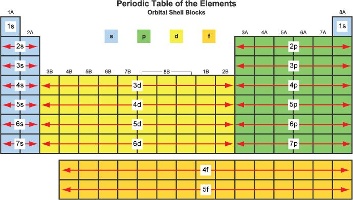
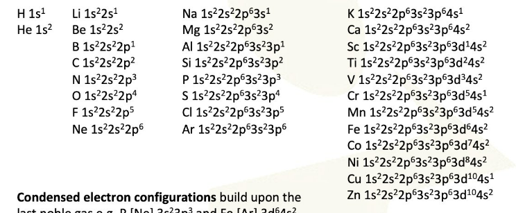
A fundamental principle governing the electron configurations of atoms is that a filled sublevel represents the most stable state, followed by a half-filled sublevel, which is more stable than a partially filled sublevel. To achieve maximum stability, which corresponds to the lowest energy state, electrons may sometimes be promoted from the s sublevel to the d sublevel. This phenomenon is particularly evident in elements belonging to Group 6B and Group 11B of the periodic table. For instance, chromium (Cr), which is in Group 6B, exhibits an electron configuration of [Ar] 4s¹3d⁵ instead of the expected [Ar] 4s²3d⁴. Similarly, copper (Cu), in Group 11B, has a configuration of [Ar] 4s¹3d¹⁰ rather than [Ar] 4s²3d⁹. This electron promotion allows for a half-filled 3d sublevel in chromium and a fully filled 3d sublevel in copper, both of which are more stable arrangements. When transition metals form ions, the electrons from the s sublevel are removed first because they require less energy to ionize compared to the electrons in the d sublevel.

Coloration in Transition Metal Complexes

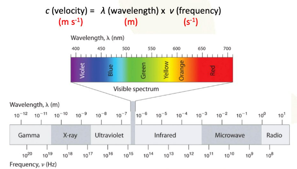
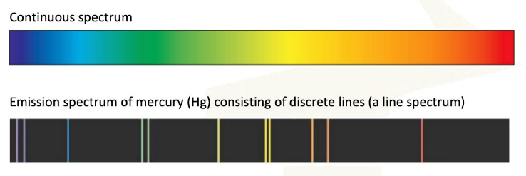
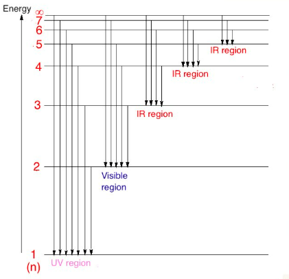
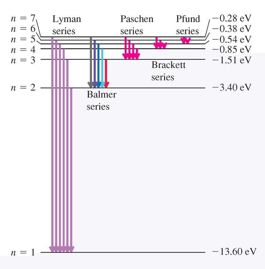
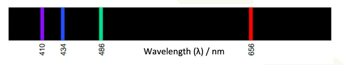
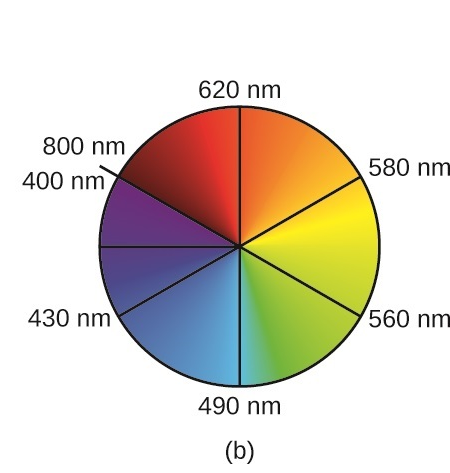
The vibrant colors often observed in transition metal compounds are directly linked to the presence of unpaired electrons in their d sublevels and their interaction with ligands. When white light passes through a solution containing a transition metal ion, certain wavelengths of light are absorbed by the d-orbital electrons. This absorption causes the electrons to jump to higher energy d-orbitals, a process known as d-orbital splitting. The remaining unabsorbed wavelengths are transmitted or reflected, and these are perceived as the color of the compound. The color observed is complementary to the color of the light absorbed. For example, consider copper and its ions:

• Copper (Cu) in its elemental form has a configuration of [Ar] 4s¹3d¹⁰ and is colored.
• The Cu⁺ ion has a configuration of [Ar] 4s⁰3d¹⁰. Since its d sublevel is completely filled, it typically does not exhibit color.
• The Cu²⁺ ion has a configuration of [Ar] 4s⁰3d⁹. The presence of an unpaired electron in the partially filled d sublevel allows for d-d transitions, resulting in a characteristic color.

In contrast, elements like zinc (Zn) and its ion Zn²⁺ do not typically display color.

• Zinc (Zn) has a configuration of [Ar] 4s²3d¹⁰.
• The Zn²⁺ ion has a configuration of [Ar] 4s⁰3d¹⁰.

Both Zn and Zn²⁺ have fully filled d sublevels, meaning there are no empty d orbitals for electrons to transition into, and thus no d-d transitions occur, leading to a lack of color.

Defining Transition Elements

It is important to note that the definition of a transition element specifically refers to an element that forms at least one ion with a partially filled d sublevel. Based on this definition, zinc (Zn) is technically not considered a transition element because both its neutral atom and its common ion (Zn²⁺) have a completely filled d sublevel.